rstoolbox.plot.plot_96wells¶

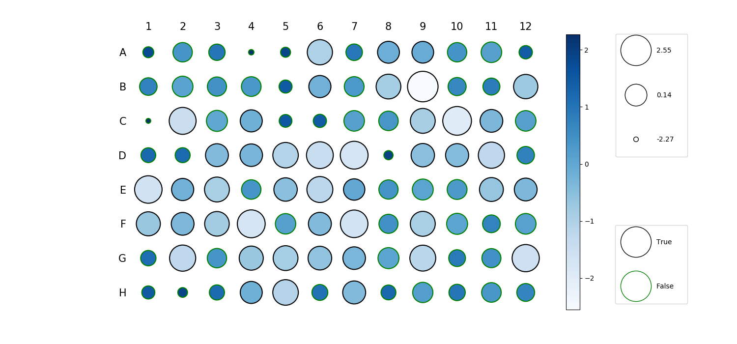
rstoolbox.plot.plot_96wells(cdata=None, sdata=None, bdata=None, bcolors=None, bmeans=None, **kwargs)¶

Plot data of a 96 well plate into an equivalent-shaped plot.

Allows up to three data sources at the same time comming from experiments performed in a 96 wells microplate. Two of this data sources can have to be numerical, and are represented as color and size, while an extra boolean dataset can be represented by the color of the border of each well.

Plot is based on scatter(); some graphical properties to control the visuals (such as cmap), can be provided through this function.

Parameters:	cdata (DataFrame) – Data contentainer to be represented by color coding. Has to contain 8 rows and 12 columns, like the 96 well plate. Contains continuos numerical data. sdata (DataFrame) – Data contentainer to be represented by size coding. Has to contain 8 rows and 12 columns, like the 96 well plate. Contains continuos numerical data. bdata (DataFrame) – Data contentainer to be represented by the edge color. Has to contain 8 rows and 12 columns, like the 96 well plate. Contains boolean data. bcolors (list() of str) – List of the two colors to identify the differences in the border for binary data. It has to be a list of 2 colors only. First color represents True instances while the second color is False. Default is black and green. bmeans (list() of str) – List with the meanings of the boolean condition (for the legend). First color represents True instances while the second color is False. Default is True and False.
Returns:	Union[Figure, Axes]
Raises:	ValueError: If input data is not a DataFrame. ValueError: If DataFrame do not has the proper shape. ValueError: If bcolors of bmeans are provided with sizes different than 2.

Example

In [1]: from rstoolbox.plot import plot_96wells
   ...: import numpy as np
   ...: import pandas as pd
   ...: import matplotlib.pyplot as plt
   ...: np.random.seed(0)
   ...: df = pd.DataFrame(np.random.randn(8, 12))
   ...: fig, ax = plot_96wells(cdata = df, sdata = -df, bdata = df<0)
   ...: plt.subplots_adjust(left=0.1, right=0.8, top=0.9, bottom=0.1)
   ...: 

In [2]: plt.show()

In [3]: plt.close()